Custom Distributions

You might want to model input uncertanty with a distribution not currenlty available in Golem. In this case you can create your own class implementing such distribution.

Here, we will reimplement a uniform distribution as a toy example.

from golem import *

import numpy as np
import pandas as pd
from matplotlib import pyplot as plt
import matplotlib
%matplotlib inline

import seaborn as sns
sns.set(context='talk', style='ticks')

To create your own distribution class to be used in Golem, you need to create a class that:

1. Inherits from the BaseDist class;

2. Implements a cdf method that returns the cumulative density for the distribution of interest. The cdf method needs to to take in two arguments, x and loc. loc is the location of the distribution, e.g. the mean for a Gaussian, and x is where the CDF needs to be evaluated at.

In addition, even though this is not required for the code to run, the __init__ method should allow to define the scale of the distribution. In the example below, we allow the user to define the range of the uniform. For a Gaussian distribution this would be the standard deviation, and so on.

# Here is a custom, user-implemented, uniform distribution class

class MyDistribution(BaseDist):

    def __init__(self, urange):
        self.urange = urange


    def cdf(self, x, loc):
        """Cumulative density function.

        Parameters
        ----------
        x : float
            The point where to evaluate the cdf.
        loc : float
            The location of the Uniform distribution.

        Returns
        -------
        cdf : float
            Cumulative density evaluated at ``x``.
        """
        a = loc - 0.5 * self.urange
        b = loc + 0.5 * self.urange

        # calc cdf
        if x < a:
            return 0.
        elif x > b:
            return 1.
        else:
            return (x - a) / (b - a)

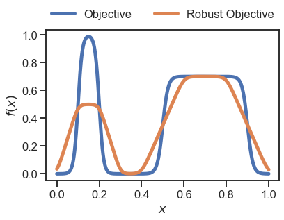
To demonstrate how this can be used, we use a simple objective function and we will compute its robust counterpart using the Uniform class available in Golem as well as the above, user-defined equivalent MyDistribution.

# a sample 1d objective function
def objective(x):

    def sigmoid(x, l, k, x0):
        return l / (1 + np.exp(-k*(x-x0)))

    sigs = [sigmoid(x,  1, 100, 0.1),
            sigmoid(x, -1, 100, 0.2),
            sigmoid(x,  0.7, 80, 0.5),
            sigmoid(x, -0.7, 80, 0.9)
           ]
    return np.sum(sigs, axis=0)

First, using the Golem.Uniform class…

# take 1000 samples in x
x = np.linspace(0, 1, 1000)

# compute objective
y = objective(x)

# compute robust objective with Golem
golem = Golem(goal='max', random_state=42, nproc=1)
golem.fit(X=x.reshape(-1,1), y=y)

# use the Golem.Uniform class here
dists = [Uniform(0.2)]
y_robust = golem.predict(X=x.reshape(-1,1), distributions=dists)

# plot results
plt.plot(x, y, linewidth=5, label='Objective')
plt.plot(x, y_robust, linewidth=5, label='Robust Objective')

_ = plt.legend(loc='lower center', ncol=2, bbox_to_anchor=(0.5 ,1.), frameon=False)
_ = plt.xlabel('$x$')
_ = plt.ylabel('$f(x)$')

[INFO] Golem ... 1 tree(s) parsed in 53.26 ms ...
[INFO] Golem ... Convolution of 1000 samples performed in 6.25 ms ...

…then with our new custom MyDistribution class:

# use MyDistribution for the prediction/convolution
dists = [MyDistribution(0.2)]
y_robust = golem.predict(X=x.reshape(-1,1), distributions=dists)

# plot the results
plt.plot(x, y, linewidth=5, label='Objective')
plt.plot(x, y_robust, linewidth=5, label='Robust Objective')

_ = plt.legend(loc='lower center', ncol=2, bbox_to_anchor=(0.5 ,1.), frameon=False)
_ = plt.xlabel('$x$')
_ = plt.ylabel('$f(x)$')

[INFO] Golem ... Convolution of 1000 samples performed in 297.95 ms ...

As you can see, the result above (orange line) obtained with the user-defined uniform is the same to that obtained with Golem.Uniform as expected.

However, note that while with Golem.Uniform the 1000 samples were processed in less than 10 ms, with MyDistribution it took almost 300 ms (~30 times slower). This is because the method cdf is called many times (about 1 million times in this example) and Golem.Uniform is implemented in Cython rather than Python. Therefore, if the execution time of the predict method in Golem with your custom distribution is too slow, you shuold consider a Cython implementation.